Random forests in QGIS: the gateway drug to GeoAI

Part 8 of the GeoAI series

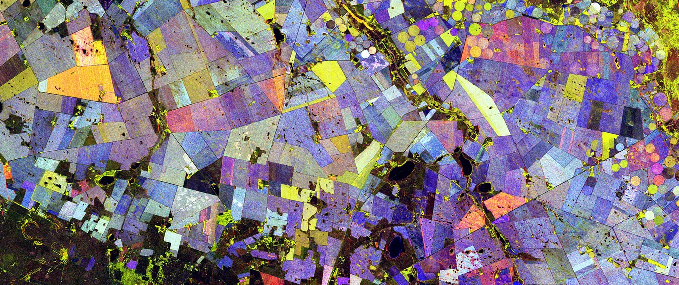
Glacial lakes in Peru’s Vilcanota range, photographed from the International Space Station. Purely for the view — though a classified raster with distinct color-coded classes ends up looking a little like this too, once you’ve run one.

Get GeoAI Frontier’s stories in your inbox

Join Medium for free to get updates from this writer.

Remember me for faster sign in

If you’ve read the rest of this series and are wondering where to actually type something into a computer, this is the article. Random Forest classification in QGIS is the easiest on-ramp into GeoAI that exists: no code, a plugin does the heavy lifting, and you get a visible result in minutes. It also happens to be the same core algorithm sitting underneath a meaningful share of production land cover and crop mapping pipelines, so the intuition you build here transfers directly.

Why Random Forest specifically

A Random Forest is an ensemble of decision trees, each trained on a slightly different random subset of your training data and features, with the final prediction coming from a vote across all of them. Three properties make it the natural starting point over other classifiers:

• It’s forgiving. It handles noisy or correlated input bands reasonably well and rarely needs much hyperparameter tuning to get a usable result on the first try.
• It gives you feature importance for free, so after classifying you can see which spectral bands or indices actually mattered — useful feedback if you’re new to which bands carry which information.
• It’s the default recommendation in nearly every accessible classification plugin, which means good documentation and a large community that’s already hit the common problems.

The worked example

You’ll need QGIS with the dzetsaka plugin, a raster (a Sentinel-2 composite works well), and a vector layer of training polygons with a field indicating class.

1. Install dzetsaka: Plugins → Manage and Install Plugins → search “dzetsaka” → Install.
2. Digitize training polygons: create a new vector layer, add an integer field (call it class), and draw a handful of small polygons over areas you can visually confirm — water, vegetation, bare ground, built-up. Five to ten polygons per class is enough to start.
3. Open the dzetsaka toolbar, select your raster as the image, your training layer as the ROI (region of interest), and class as the field.
4. Set the classifier to Random Forest and leave the default parameters (100 trees is a common default) — they’re a reasonable starting point.
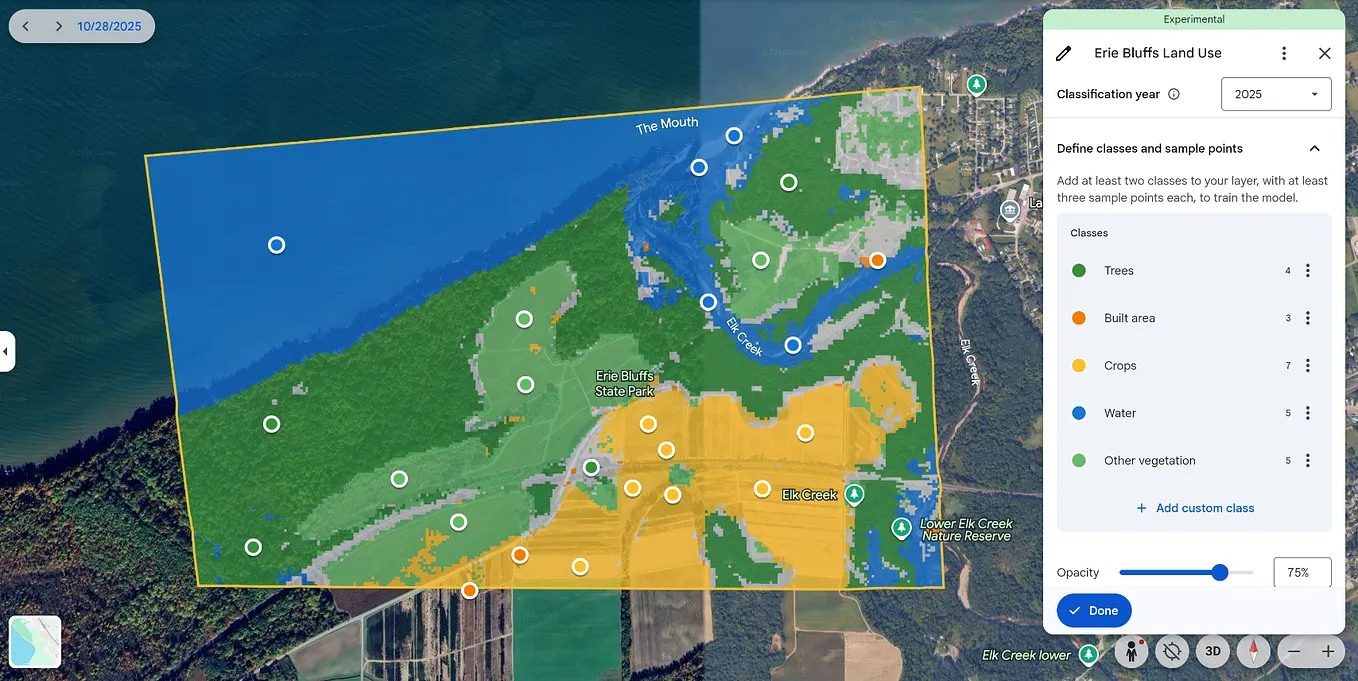
5. Run it. dzetsaka trains the model and classifies the entire raster in the same step, producing a new classified layer, usually within seconds to a couple of minutes depending on raster size.

That’s the whole workflow, shown below.

What to look at afterward

Once you have a classified raster, two things are worth checking before you trust it:

• Visual sanity check: does water look like water, does vegetation look like vegetation? Obvious misclassifications at this stage usually mean a training polygon was drawn somewhere ambiguous, or a class is spectrally too similar to another (shadow and water are a classic confusion pair).
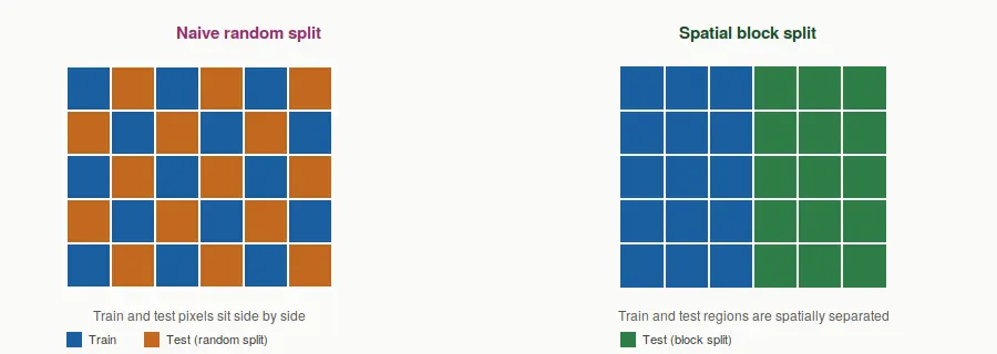
• Accuracy assessment, if you have separate validation points: dzetsaka and the Semi-Automatic Classification Plugin both include tools for this. Don’t validate against the same polygons you trained on — that number will look great and mean very little, for the same reason discussed in the previous article on validation strategy.

Why this is the gateway, not the destination

Everything covered in this series so far — training data as labeled examples, the model as a rulebook, prediction as applying that rulebook broadly — is exactly what just happened inside dzetsaka, just wrapped in a UI that hides the code. The moment you’re comfortable with this workflow, you’ve already internalized the core loop that every more sophisticated GeoAI pipeline repeats: get representative labeled examples, train something, apply it broadly, then check honestly whether it worked.

What changes as you move toward deep learning is mostly what’s doing the learning — a neural network instead of a forest of decision trees — and how the input is packaged, which is exactly the pixel-to-tensor translation covered a couple of articles back. The underlying loop doesn’t change nearly as much as the tooling makes it feel like it should.