Model Evaluation Metrics in Machine Learning: Regression and Classification Explained

Understand MAE, MSE, RMSE, R² Score, Accuracy, Precision, Recall, F1-Score, ROC-AUC, and Log Loss with simple explanations, formulas, and Python examples.

Introduction

In Machine Learning, building a model is only the first step. We also need to evaluate how well the model performs on unseen data.
Model evaluation metrics are measurements used to understand how accurately a model makes predictions and where it makes mistakes.
For example:

• If we predict house prices, we need to measure how far the predicted prices are from the actual prices.
• If we classify emails as spam or not spam, we need to measure how many predictions are correct and how many spam emails are missed.

Different Machine Learning tasks require different evaluation metrics.

1. Regression Metrics

Regression is used when the target variable is a continuous numerical value, such as house prices, sales, temperature, or salary.
Common regression metrics include:

• MAE (Mean Absolute Error): Measures the average absolute difference between actual and predicted values.
• MSE (Mean Squared Error): Calculates the average of squared prediction errors.
• RMSE (Root Mean Squared Error): Takes the square root of MSE and expresses the error in the target variable’s units.
• R² Score: Measures how well the model explains variation in the target variable compared with a baseline that predicts the mean.
• Adjusted R²: Adjusts R² based on the number of predictors and observations, making it useful when comparing certain regression models.

For error metrics such as MAE, MSE, and RMSE, lower values generally indicate better predictions. For R² and Adjusted R², higher values generally indicate a better fit, but the metrics should be interpreted in context.

2. Classification Metrics

Classification is used when the target variable represents a category, such as spam or not spam, positive or negative, or approved or rejected.

Common classification metrics include:

• Accuracy: Measures the proportion of all predictions that are correct.
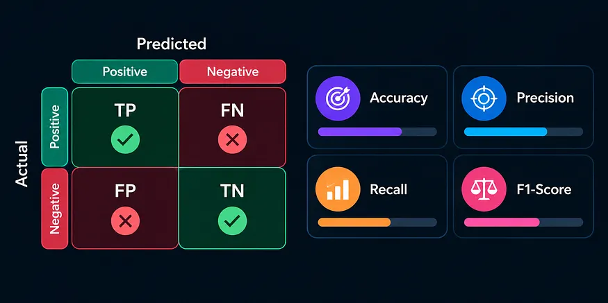
• Confusion Matrix: Summarizes correct and incorrect predictions using True Positives, True Negatives, False Positives, and False Negatives.
• Precision: Measures how many predicted positive cases are actually positive.
• Recall: Measures how many actual positive cases the model correctly identifies.
• F1-Score: Combines precision and recall into a single score using their harmonic mean.
• ROC-AUC: Evaluates how well a model distinguishes between positive and negative classes across different classification thresholds.
• Log Loss: Measures the quality of predicted probabilities and penalizes confident incorrect predictions.

Accuracy alone may not be enough when a dataset is imbalanced. For example, if only 2% of transactions are fraudulent, a model that predicts every transaction as legitimate could achieve 98% accuracy while detecting no fraud.

Why Are Evaluation Metrics Important?

Evaluation metrics help us:

1. Compare different Machine Learning models.
2. Identify the strengths and weaknesses of a model.
3. Understand the types of prediction errors a model makes.
4. Select a model that suits the real-world problem.
5. Monitor model performance and improve prediction

Regression Metrics →MAE, MSE, RMSE, R² Score, and Adjusted R²

Regression metrics help us measure how closely a model’s predicted numerical values match the actual values. They are commonly used for problems such as house price prediction, sales forecasting, and salary prediction.

Let’s understand five important regression metrics.

1. MAE (Mean Absolute Error)

Mean Absolute Error (MAE) measures the average absolute difference between actual values and predicted values.

It tells us, on average, how far the model’s predictions are from the actual values.

Formula:

Where:

• n= number of data points
• yi= actual value
• y^i = predicted value
• yi-y^i = absolute prediction error

Key points:

• Lower MAE generally indicates better predictions.
• MAE uses the same units as the target variable.
• It is less sensitive to large errors than MSE because it does not square the errors.

2. MSE (Mean Squared Error)

Mean Squared Error (MSE) measures the average of the squared differences between actual and predicted values.
Squaring the errors gives larger errors a greater influence on the final score.

Formula:

Key points:

• Lower MSE generally indicates better predictions.
• Large errors receive a much greater penalty.
• MSE is expressed in squared units of the target variable.
• It is sensitive to outliers because their errors are squared.

3. RMSE (Root Mean Squared Error)

Root Mean Squared Error (RMSE) is the square root of MSE. It measures prediction error in the same units as the target variable.

Formula:

Key points:

• Lower RMSE generally indicates better predictions.
• It uses the same units as the target variable.
• Like MSE, it penalizes large errors more heavily than MAE.
• RMSE is useful when we want an error measure that is easier to interpret in the original units.

Which should you choose?

• Use MAE when you want a straightforward average error and less sensitivity to outliers.
• Use MSE when large errors should receive a stronger penalty.
• Use RMSE when you want to penalize large errors but interpret the result in the target’s original units.

4. R² Score (Coefficient of Determination)

R² Score measures how well a regression model explains the variation in the target variable compared with a baseline that predicts the target’s mean.

Formula:

Where:

• y_i = actual value
• y^i= predicted value
• y_ = mean of the actual values

How to interpret R²:

• R² = 1: Perfect predictions on the evaluated data.
• R² = 0: The model performs as well as the mean-prediction baseline under the standard definition.
• R² = 0.80: The model explains 80% of the variation relative to that baseline.
• R² below 0: The model performs worse than the mean-prediction baseline on the evaluated data.

Important: R² is not always between 0 and 1. It can be negative, particularly when evaluating a model on unseen test data.
A higher R² can indicate a better fit, but it does not guarantee that a model will generalize well to new data.

5. Adjusted R²

Adjusted R² is a modified version of R² that accounts for the number of predictors and observations. It is especially useful when comparing regression models that use different numbers of independent variables.
Unlike ordinary R², which cannot decrease when additional predictors are added to a standard least-squares regression model fitted on the same data, Adjusted R² can decrease when a new predictor does not improve the model enough to justify its inclusion.

Get Gollapalli Sai Teja’s stories in your inbox

Join Medium for free to get updates from this writer.

Remember me for faster sign in

Formula:

Where:

• (R²) = ordinary R² score
• (n) = number of observations
• (p) = number of independent variables or predictors

Key points:

• It accounts for the number of predictors.
• It helps compare models with different numbers of predictors.
• A new predictor may increase ordinary R² but decrease Adjusted R².
• It is commonly used in regression analysis, especially when comparing linear regression models.

Adjusted R² should not be treated as a substitute for evaluating performance on unseen data.

Python Implementation Using Scikit-Learn

We can calculate all five metrics using Python’s scikit-learn library.

from sklearn.metrics import (
mean_absolute_error,
mean_squared_error,
r2_score)
import numpy as np

# Actual and predicted values
y_actual = np.array([100, 150, 200])
y_predicted = np.array([110, 140, 180])

# Regression metrics
mae = mean_absolute_error(y_actual, y_predicted)
mse = mean_squared_error(y_actual, y_predicted)
rmse = np.sqrt(mse)
r2 = r2_score(y_actual, y_predicted)

print("MAE:", mae)
print("MSE:", mse)
print("RMSE:", rmse)
print("R² Score:", r2)

# Adjusted R²
n = len(y_actual)
p = 1 # Number of predictors

adjusted_r2 = 1 - (1 - r2) * (n - 1) / (n - p - 1)
print("Adjusted R²:", adjusted_r2)

Note: The example uses only three observations to demonstrate the calculations. Adjusted R² is meaningful only when the sample size and number of predictors make the formula valid ((n>p+1)); in practice, use a larger dataset for model evaluation.

Confusion Matrix in Machine Learning

A Confusion Matrix is a table used to evaluate a classification model by comparing its predicted labels with the actual labels.
It shows how many predictions are correct and how many are incorrect. It is also used to calculate accuracy, precision, recall, and F1-score.
For example, suppose we build a Machine Learning model to predict whether an email is spam or not spam.

Understanding the Confusion Matrix

For a binary classification problem, the confusion matrix contains four important values:

Predicted Negative:-
Actual Negative →True Negative (TN)
Actual Positive →False Negative (FN)

Predicted Positive:-
Actual Negative →False Positive (FP)
Actual Positive → True Positive (TP)

1. True Positive (TP)

The model predicts Positive, and the actual class is also Positive.
Example: A spam email is correctly identified as spam.

2. True Negative (TN)

The model predicts Negative, and the actual class is also Negative.
Example: A normal email is correctly identified as not spam.

3. False Positive (FP)

The model predicts Positive, but the actual class is Negative.
Example: A normal email is incorrectly classified as spam.
This is also called a Type I error.

4. False Negative (FN)

The model predicts Negative, but the actual class is Positive.
Example: A spam email is incorrectly classified as not spam.
This is also called a Type II error.

A Simple Numerical Example

Suppose a classification model evaluates 100 emails and produces these results:
Predicted Not SpamPredicted SpamActual Not Spam40 (TN)10 (FP)Actual Spam5 (FN)45 (TP)
From this matrix:

• TP = 45: Spam emails correctly identified as spam.
• TN = 40: Normal emails correctly identified as not spam.
• FP = 10: Normal emails incorrectly identified as spam.
• FN = 5: Spam emails incorrectly identified as not spam.

The model made 85 correct predictions out of 100: 45 true positives and 40 true negatives.

These four values form the foundation for many classification metrics.

Python Implementation Using Scikit-Learn

We can create a confusion matrix using confusion_matrix() from sklearn.metrics

from sklearn.metrics import confusion_matrix
# Actual labels: 0 = Not Spam, 1 = Spam
y_actual = [0, 0, 0, 0, 0, 0, 1, 1, 1, 1]
# Predicted labels
y_predicted = [0, 0, 0, 0, 1, 1, 0, 1, 1, 1]
cm = confusion_matrix(y_actual, y_predicted, labels=[0, 1])
print(cm)

Why Is the Confusion Matrix Important?

• It shows the types of mistakes a model makes.
• It helps identify false positives and false negatives.
• It provides the values needed to calculate precision, recall, and F1-score.
• It is particularly useful when accuracy alone does not describe model performance adequately.

Accuracy, Precision, and Recall

After understanding the confusion matrix, we can use its four values — True Positive (TP), True Negative (TN), False Positive (FP), and False Negative (FN) — to calculate important classification metrics.
Let’s use the spam email example from the previous section.

1. Accuracy

Accuracy measures the proportion of all predictions that the model classifies correctly.

Formula:

When should we use accuracy?

Accuracy is useful when the classes are reasonably balanced and false positives and false negatives have similar consequences.
Limitation: Accuracy can be misleading for imbalanced datasets. For example, if only 2 out of 100 transactions are fraudulent, a model that predicts every transaction as legitimate achieves 98% accuracy but detects no fraud.

2. Precision

Precision measures how many of the cases predicted as positive are actually positive.

In simple words, precision answers:

Of all the cases the model predicted as positive, how many were truly positive?

Formula:

When is precision important?

Precision is especially important when false positives are costly.
For example, a legitimate email incorrectly sent to the spam folder may cause the user to miss an important message. A high-precision model reduces these false alarms.

3. Recall (Sensitivity)

Recall, also known as Sensitivity or True Positive Rate (TPR), measures how many actual positive cases the model correctly identifies.
In simple words, recall answers:
Of all the cases that were truly positive, how many did the model find?

Formula:

When is recall important?

Recall is especially important when missing a positive case has serious consequences.
For example, in fraud detection or disease screening, a false negative may be costly. A high-recall model aims to identify more of the actual positive cases, although it may also produce more false positives.

Python Implementation Using Scikit-Learn

We can calculate accuracy, precision, and recall using sklearn.metrics.
from sklearn.metrics import ( accuracy_score, precision_score,recall_score)
# 0 = Not Spam, 1 = Spam
y_actual = [0, 0, 0, 0, 0, 0, 1, 1, 1, 1]
y_predicted = [0, 0, 0, 0, 1, 1, 0, 1, 1, 1]
accuracy = accuracy_score(y_actual, y_predicted)
precision = precision_score( y_actual, y_predicted, zero_division=0)
recall = recall_score( y_actual, y_predicted, zero_division=0)print("Accuracy:", accuracy)
print("Precision:", precision)
print("Recall:", recall)

Key Takeaway

• Accuracy measures overall correctness.
• Precision focuses on the correctness of positive predictions.
• Recall focuses on finding actual positive cases.

Always choose evaluation metrics based on the problem, class distribution, and cost of different types of mistakes. A model with high accuracy is not necessarily the best model for every real-world application.

F1-Score

F1-Score combines Precision and Recall into a single metric using their harmonic mean. It is useful when we need to balance correctly identifying positive cases with avoiding false positive predictions.

Formula:

• Higher F1-Score: Generally indicates a better balance between precision and recall.
• When to use it: When both false positives and false negatives matter, especially with imbalanced datasets.
• Important: Always check precision and recall separately when different types of errors have different costs.

ROC Curve and AUC

The ROC (Receiver Operating Characteristic) Curve is a graph used to evaluate a binary classification model at different classification thresholds.
AUC (Area Under the Curve) measures how well the model distinguishes between positive and negative classes.

Important Terms

• TPR (True Positive Rate): The proportion of actual positive cases correctly identified. It is the same as Recall.
• FPR (False Positive Rate): The proportion of actual negative cases incorrectly predicted as positive.

Formulas:
TPR=TP(TP+FN)

FPR=FP(FP+TN)
The ROC curve plots TPR against FPR at different thresholds.

How to Interpret AUC

• AUC = 1.0: Perfect separation of positive and negative cases.
• AUC = 0.5: No better than random ranking in the usual binary setting.
• AUC below 0.5: Worse-than-random ranking, which may indicate that the model’s scores rank the classes in the wrong direction.

A higher AUC generally indicates better ability to distinguish between the classes.

from sklearn.metrics import roc_auc_score, roc_curve
y_actual = [0, 0, 1, 1]
y_scores = [0.1, 0.4, 0.35, 0.8]
auc = roc_auc_score(y_actual, y_scores)
fpr, tpr, thresholds = roc_curve(y_actual, y_scores)
print("ROC-AUC:", auc)

Conclusion

Model evaluation metrics help us understand how well a Machine Learning model performs and whether its predictions are useful for a real-world problem.
For regression, MAE, MSE, RMSE, R², and Adjusted R² help evaluate numerical predictions. For classification, accuracy, precision, recall, F1-Score, ROC-AUC, and Log Loss provide different ways to evaluate predicted classes and probabilities.
The key takeaway is that no single metric is best for every problem. Choose metrics based on the type of task, the balance between classes, and the cost of different prediction errors.
Understanding these metrics helps us compare models, identify weaknesses, and make better Machine Learning decisions.